install.packages("RiskMap")1 Introduction
The purpose of this book is to demonstrate how to conduct model-based geostatistical analysis of public health data using the RiskMap R package. In this introductory chapter, we outline the prerequisites for using the book, its learning objectives, and the required software. We then provide a brief overview of the class of models that will be covered and the real-world examples that will be used to illustrate the methods and software.
1.1 Objectives of this book
The overall aim of this book is to equip you with the skills needed to perform geostatistical analyses of public health data within the R software environment. As you progress through the material, you will learn how to explore geostatistical datasets using graphical procedures and summary statistics, to formulate and fit geostatistical models by maximum likelihood estimation, to generate predictions of health outcomes at different spatial scales, to visualize and interpret the resulting outputs, to model relationships between spatially referenced risk factors and health outcomes, and to evaluate model assumptions while assessing predictive performance. Although the emphasis is on public health, the statistical concepts and software tools presented here are broadly applicable to geostatistical data from many other scientific fields.
1.2 Prerequisites
To make the most of this book, readers are expected to have prior knowledge of three areas: probability, statistics, and R programming. The following sections describe the essential background in each area.
1.2.1 Topics in probability
A working knowledge of probability is important to understand the material covered in this book. You should already be familiar with the definitions and properties of continuous and discrete distributions, with the use of means, variances and skewness to describe their properties, and with the concepts of stochastic dependence and correlation, including the distinction between marginal and conditional distributions. It is also important to understand the properties of the Gaussian, Binomial and Poisson distributions, and to be aware of the definition and key properties of the multivariate Gaussian distribution. A clear introduction to these topics, with worked examples, can be found in Ross (2013).
1.2.2 Topics in statistics
Statistical modelling provides the theoretical foundation for this book, which relies heavily on likelihood-based inference and, in particular, maximum likelihood estimation. You should therefore be comfortable with the use of point and interval estimation within this framework. Because the geostatistical modelling approach builds directly on Generalized Linear Models (GLMs), prior knowledge of GLMs is essential. We recommend reviewing the theory and applications of linear regression for continuous outcomes, Binomial regression and Poisson regression for count data. This book will build on those foundations with geostatistical models for continuously measured outcomes and counts. A comprehensive overview of GLMs and their implementation in R is given in Dobson and Barnett (2008). For further background on likelihood-based inference, see chapters 1, 2 and 4 of Pawitan (2001).
1.2.3 Topics in R programming
Although advanced programming skills are not required, a working knowledge of R is necessary. You should already be able to create and manipulate vectors and matrices, use logical and character variables, work with lists and data frames, import data into R, and produce basic plots. A wide range of freely available material covers these topics; a useful starting point is An Introduction to R, available at https://cran.r-project.org/manuals.html.
1.3 Obtaining and running the R packages
It is advised that you obtain the latest 64-bit version of R in order to run the R code of this book. To install R, go to the R website, where you can download the installer packages for Windows and Mac, and find instructions for Linux, using binary files.
The list of the R packages used in this book is provided in Table 1.1.
| R packages | Used for |
|---|---|
RiskMap (E) |
Estimation of geostatistical models and spatial prediction |
lme4 |
Estimation of generalized linear mixed models |
sf (E) |
Handling of spatial data in R |
terra (E) |
Handling of raster files in R |
ggplot2 (E) |
Creating maps and exploratory plots |
dplyr (E) |
Data wrangling and manipulation |
tidyr (E) |
Reshaping and tidying data |
rgeoboundaries (R) |
Accessing global administrative boundary datasets from GeoBoundaries |
gridExtra (R) |
Arranging multiple plots and tables in a grid layout |
patchwork (R) |
Combining multiple ggplot2 plots into a single coherent display |
factoextra (R) |
Extracting and visualizing multivariate analysis results |
scales (R) |
Controlling axis transformations, breaks, and labels in ggplot2 graphics |
crsuggest (R) |
Guessing coordinate reference systems when unknown |
Note
When running the code examples in this book, you may occasionally encounter error messages indicating that a function cannot be found. This usually happens when the corresponding R package has not been loaded. To avoid such issues, we recommend always loading all the packages listed in Table 1.1 before running the code.
To install packages in R for the first time, you can use the command install.packages in the R console. For example, to install the stable CRAN release of the RiskMap package, run:
Alternatively, you can install the development version of RiskMap from GitHub, which is updated more frequently but should be considered a testing version. This requires the remotes package:
install.packages("remotes")
remotes::install_github("giorgistat/RiskMap")
1.4 Data-sets used in the book
In this book, we use data available from the RiskMap package. These data-sets are grouped into two categories: examples, which are used to demonstrate the application of R functions and modelling steps, and case studies, which are analysed in greater depth to illustrate the use of complete geostatistical workflows. In this introductory chapter, we focus on presenting the example data-sets, while leaving the detailed presentation and analysis of the case study data-sets to Chapter 5.
Each of the data-sets, whether example or case-study, can be loaded directly from the RiskMap package using the command:
data(NAME_OF_THE_DATASET)where NAME_OF_THE_DATASET should be replaced with the name of one of the data-sets listed in Table 1.2.
RiskMap package. Data-sets listed as “Example” are used throughout the book to illustrate the use of R functions. Data-sets listed as “Case study” are analysed in Chapter 5.
| Names of the data-set | Short description | Used in this book as |
|---|---|---|
galicia |
Lead concentration measured from moss samples collected in Galicia, Northern Spain | Example |
liberia |
Prevalence data on river blindness from Liberia | Example |
malkenya |
Malaria prevalence data from a community and school survey conducted in Western Kenya | Example |
italy_sim |
Simulated geostatistical data within the Italian national boundaries | Example |
malnutrition |
Data on stunting among children in Ghana | Case study |
infect_sma |
West Nile virus infection prevalence in Culex pipiens mosquitoes from the Sacramento Metropolitan Area, USA | Case study |
abund_sma |
Abundance of Culex pipiens mosquitoes from the Sacramento Metropolitan Area, USA | Case study |
1.4.1 Lead concentration in Galicia
Lead is a heavy metal that, at high concentrations, can cause chronic damage to living organisms over prolonged periods. For this reason, its distribution and sources require regular monitoring. A common approach is to measure lead concentrations in plants, which act as bioindicators of environmental contamination. The data considered here (Figure 1.1) consist of measurements from 132 moss samples collected in the year 2000 in and around Galicia, a region in north-western Spain. One of the main objectives of the survey was to map the spatial distribution of lead concentration in order to identify potential sources of contamination; for further details, see Fernández, Rey, and Carballeira (2000).
Geostatistical modelling provides a framework for predicting lead concentrations across Galicia and for distinguishing between random variation, for instance due to measurement error, and genuine spatial variation, which is the principal focus of analysis.
This dataset will be used throughout the book to illustrate the spatial analysis of continuously measured variables using linear geostatistical models.
1.4.2 River-blindness in Liberia
In low-resource settings, where disease registries are often absent, cross-sectional surveys provide a critical tool for estimating disease burden in the population of interest. The data considered in this example (Figure 1.2) were collected as part of the Rapid Epidemiological Mapping of Onchocerciasis (REMO), an Africa-wide initiative conducted in 2011 across 20 countries (Zouré et al. 2014). The purpose of REMO was to identify areas where river blindness (onchocerciasis)—a parasitic disease transmitted by black flies that breed along fast-flowing rivers—remains a public health problem. Of particular concern are communities with prevalence above 20%, which are prioritised for treatment
In this book, we use data collected in Liberia to model nodule prevalence, which measures the proportion of individuals in a population presenting with palpable nodules under the skin. These nodules are formed around adult Onchocerca volvulus worms, the parasite responsible for river blindness. Because detecting nodules through a simple physical examination is far less costly and logistically demanding than laboratory-based or molecular diagnostic methods, nodule prevalence serves as a practical and widely used proxy for estimating infection burden in large-scale epidemiological surveys, such as REMO.
Through this dataset, we demonstrate how to formulate and fit Binomial geostatistical models and how these can be applied to predict prevalence across a region of interest.
1.4.3 Malaria in the Western Kenyan Highlands
Malaria is among the deadliest infectious diseases affecting populations in tropical and subtropical regions. It is caused by parasites of the genus Plasmodium, transmitted through the bite of infected female Anopheles mosquitoes. In the following chapters, we analyse a dataset (Figure 1.3) from a cross-sectional community survey conducted in July 2010 in Nyanza Province, in the western highlands of Kenya (Stevenson 2013).
What distinguishes this dataset from the other examples is that it contains both individual- and household-level information. The primary outcome is the result of a rapid diagnostic test for malaria. In the original study, data were collected from 46 community clusters (clearly visible as spatial groupings in Figure 1.3) each defined by a primary school and the surrounding residential compounds within approximately a 600 m radius. Each cluster therefore corresponds to a school and its adjacent community catchment area.
In this book, we show how to incorporate the hierarchical structure of the data together with the binary nature of the outcome at each stage of the geostatistical analysis.
1.4.4 Anopheles gambiae mosquitoes in Southern Cameroon
In studies of vector-borne and zoonotic diseases, understanding the vector distribution can help to better guide the decision-making process for the implementation, monitoring and evaluation of control programmes. Anopheles gambiae mosquitoes are one of the main vectors for malaria transmission in sub-Saharan Africa. Their distribution over space is affected by several environmental and climatic factors, including temperature, humidity and vegetation.
The data-set on mosquitoes (Figure 1.4) that we will use in the book consists of a sub-set taken from a larger database (Tene Fossog et al. 2015). This was assembled in order to understand how the environment affects the distribution of different species of Anopheles mosquitoes in sub-Saharan Africa. This example data-set will be used to illustrate the application of Poisson geostatistical models for mapping mosquitoes abundance.
1.4.5 Simulated-dataset
The data-set reported in Figure 1.5 was generated using a geostatistical model, with the addition of unstructured random effects at provincial and regional level. More details on how this data-set was generated will be provided in Section 3.2. Whilst this data-set does not have any scientific relevance, it will serve us to illustrate some of the more advanced features of the RiskMap package that enable the inclusion of random effects, in addition to the latent Gaussian process that is common to all geostatistical models. The skills you will acquire through the analysis of this data-set will be useful for the analysis of data-sets presented as case studies in Chapter 5.
1.5 Geostatistical problems and geostatistical models
What the examples of the previous section have in common is that, in each case, the goal of the statistical analysis is to draw inferences on an unobserved spatially continuous surface using data collected from a finite set of locations. The lead concentration in Galicia, the prevalence for river-blindness in Liberia and the abundance of A. gambiae mosquitoes in Cameroon can all be represented as spatially continuous processes that originate from the combined effects of environmental factors. We denote this class of inferential problems as geostatistical problems for which a solution can be found through the development and application of suitable geostatistical models, which are the subject of this book.
As one can soon realize, geostatistical problems are not unique to global health but arise in many other fields of science, including economics, physics, biology and geology. It thus comes to no surprise that geostatistics was initially developed in the South African mining industry in the 1950s (Krige 1951). This was then further developed as a self-contained discipline by Georges Matheron and other researchers at Fontainebleau, in France (Matheron 1963; Chilès and Delfiner 2016). In Watson (1971) and Watson (1972) a first connection is drawn between geostatistics and the prediction of stochastic processes. However, it is only with Ripley (1981) and then N. A. C. Cressie (1991) that geostatistics is explicitly brought into a classical statistical framework for the analysis of spatially referenced data. P. J. Diggle, Tawn, and Moyeed (1998) coined the term model-based geostatistics and introduced this as belonging to the general class of generalized linear mixed models (Breslow and Clayton 1993), while emphasizing the use of likelihood-based methods of inference. As in P. J. Diggle, Tawn, and Moyeed (1998), also in this book, we advocate the application of model-based geostatistical models as a class of parametric statistical models on which inference can be carried out using either maximum likelihood estimation or Bayesian methods.
More precisely, our attention will be directed at the class of generalized linear geostatistical models, or GLGMs. To formally specify this, we define the spatial stochastic process \(S(\cdot)\), representing an unobserved spatially continuous random field. For a set of locations \(X = (x_1, \ldots, x_n)\), we denote by
\[ S = (S(x_1), \ldots, S(x_n)) \]
the vector of process realizations at those locations. We also define the random vector \(Y = (Y_1, \ldots, Y_n)\), representing the outcomes observed at the same locations. Throughout, we use \([A]\) to denote “the distribution of the random variable \(A\).” To formulate a GLGM, we should then specify the joint distribution of \(S\) and \(Y\), which we write as
\[ [Y, S] = [S] [Y | S]. \tag{1.1}\]
On the right-hand side of the equation above, we have factorized the joint distribution of \(Y\) and \(S\), as the product between the marginal distribution of \(S\) and the conditional distribution of \(Y\) given \(S\). Hence, the formulation of a GLGM can be broken down into the tasks of formulating \([S]\) and \([Y | S]\).
In defining \([S]\), throughout the book, we shall assume that this is a zero-mean stationary and isotropic Gaussian process. In other words, these assumptions impose that the joint distribution of \(S(X) = (S(x_1),\ldots,S(x_n))\), i.e. the process \(S\) at the sampled locations \(x_1, \ldots, x_n\), is invariant with respect to rotations and translations of the locations \(X\). In practical terms, the main implication of this is that, for any pair of locations \(x_i\) and \(x_j\) the correlation function \(\rho(\cdot)\) between \(S(x_i)\) and \(S(x_j)\) is purely a function of the Euclidean distance, \(u_{ij}\), between \(x_i\) and \(x_j\), i.e. \[ {\rm cov}\{S(x_i), S(x_j)\} = \sigma^2\rho(u_{ij}), \tag{1.2}\]
where \(\sigma^2\) is the variance of \(S(x)\) for all \(x\). Below we provide more details on the type of covariance functions that we consider in this book. Furthermore, the fact that we assume the process \(S\) to have mean zero is because this process acts as a residual term in our modelling of \(Y\). This aspect will be reiterated several times in the following chapters, as it has important implications for the interpretation of the other components of a geostatistical model, and for understanding the results of the analysis.
Finally, we model \([Y | S]\), i.e. the distribution of \(Y\) given \(S\), as a set of mutually independent distributions which belong to the exponential family, as defined in classical generalized linear modelling framework (Nelder and Wedderburn 1972). It then follows that, we can write \([Y | S]\) as
\[ [Y | S] = \prod_{i=1}^n [Y_i | S(x_i)]. \tag{1.3}\]
The final step then consists of specifying a distribution for \([Y_i | S(x_i)]\). Table 1.3 gives the range, mean and variance of the three specifications for $[Y_i | S(x_i)]$$ which we will consider in this book. In Table 1.3, the canonical function, say \(g(\cdot)\), denotes the natural transformation of the mean component \(\mu_i\) that allows us to introduce both covariates and the spatial process \(S(x_i)\) into the model so as to explain the variation in \(\mu_i\) as
\[ g(\mu_i) = d(x_i)^\top \beta + S(x_i). \tag{1.4}\]
where \(d(x_i)\) is a vector of spatially referenced covariates with associated regression coefficients \(\beta\). Finally, the quantity \(m_i\), which appears in the formulation of the Binomial and Poisson distributions, is an offset quantity that accounts for the number of tests or the population size at a given location \(x_i\).
| Distribution | Range of \(Y_i\) | Mean of \([Y_i | S(x_i)]\) | Variance of \([Y_i | S(x_i)]\) | Canonical link |
|---|---|---|---|---|
| Gaussian | \((-\infty, +\infty)\) | \(\mu_i\) | \(\tau^2\) | \(g(\mu_i) = \mu_i\) |
| Binomial | \(1,\dots,m_i\) | \(m_i\mu_i\) | \(m_i\mu_i(1-\mu_i)\) | \(g(\mu_i) = \log\{ \mu_i/(1-\mu_i) \}\) |
| Poisson | \(1,2,\ldots,\infty\) | \(m_i\mu_i\) | \(m_i\mu_i\) | \(g(\mu_i) = \log\{ \mu_i \}\) |
Based on the formulation in (1.4), we can see that \(S(x_i)\) quantifies residual spatial effects on \(\mu_i\) that have not been accounted for by the covariates \(d(x_i)\). In an ideal scenario, the covariates \(d(x_i)\) should explain all the spatial variation without the need for \(S(x_i)\). Although this is often unrealistic, in practice we may be able to explain most of the variation in \(\mu_i\) through \(d(x_i)\) and, hence, reduce \(S(x_i)\) to a negligible component. In Chapter 2, we will show how a thorough exploratory analysis can help to understand whether we have come close to that ideal scenario or if we need to use a GLGM to model the data.
The model described in (1.4) can be seen as the most basic GLGM that can be used for a geostatistical analysis. As we will see in the analysis of some of the examples, extensions of this model will be required to accommodate the intrinsic non-spatial random variation of the data which is not captured by the covariates.
Statistical models are typically applied in two main ways: to make predictions, or to model associations that help us understand relationships between variables, whether causal or not. Most geostatistical applications fall into the first category, where the objective is to make predictive inferences about the process \(S(x)\) at locations \(x\) that are typically outside the set of sampled sites. However, as we will illustrate in later chapters, geostatistical models also play an important role in understanding associations between variables. In particular, we will show that accounting for spatial correlation can substantially affect both the point estimates and standard errors of the regression parameters \(\beta\).
1.5.1 The Matern family of correlation functions
Throughout the book, we shall consider the Matern (2013) family of correlation functions to model the spatial correlation of the Gaussian process \(S(x)\). This is defined as
\[ \rho(u;\phi,\kappa) = \{2^{\kappa-1} \Gamma(\kappa)\}^{-1} (u/\phi)^\kappa K_\kappa(u/\phi), \tag{1.5}\]
where \(\phi>0\) and \(\kappa>0\) are parameters and \(K_\kappa(\cdot)\) is the modified Bessel function of the third kind of order \(\kappa\). The parameters \(\phi\) and \(\kappa\) regulate how fast the spatial correlation decays to zero with increasing distance, and the smoothness of the process, respectively. By smoothness we mean the degree of differentiability of the underlying spatial surface: smaller values of \(\kappa\) produce rougher, less regular surfaces, whereas larger values of \(\kappa\) lead to smoother and more spatially continuous processes.
A special case of the Matern family of correlation functions, obtained when \(\kappa = 0.5\), will be of particular relevance to the applications considered in this book. This is the exponential correlation function, which we write as
\[ \rho(u;\phi) = \exp\{-u/\phi\}. \tag{1.6}\]
Another special case, which we do not consider in this book but which is often used in machine learning applications, is the Gaussian correlation function, obtained as a limiting case for \(\kappa \to +\infty\), representing the smoothest possible process within the Matérn family.
To better understand how \(\phi\) and \(\kappa\) affect the spatial correlation and the pattern of the spatial surface, we now consider some examples.
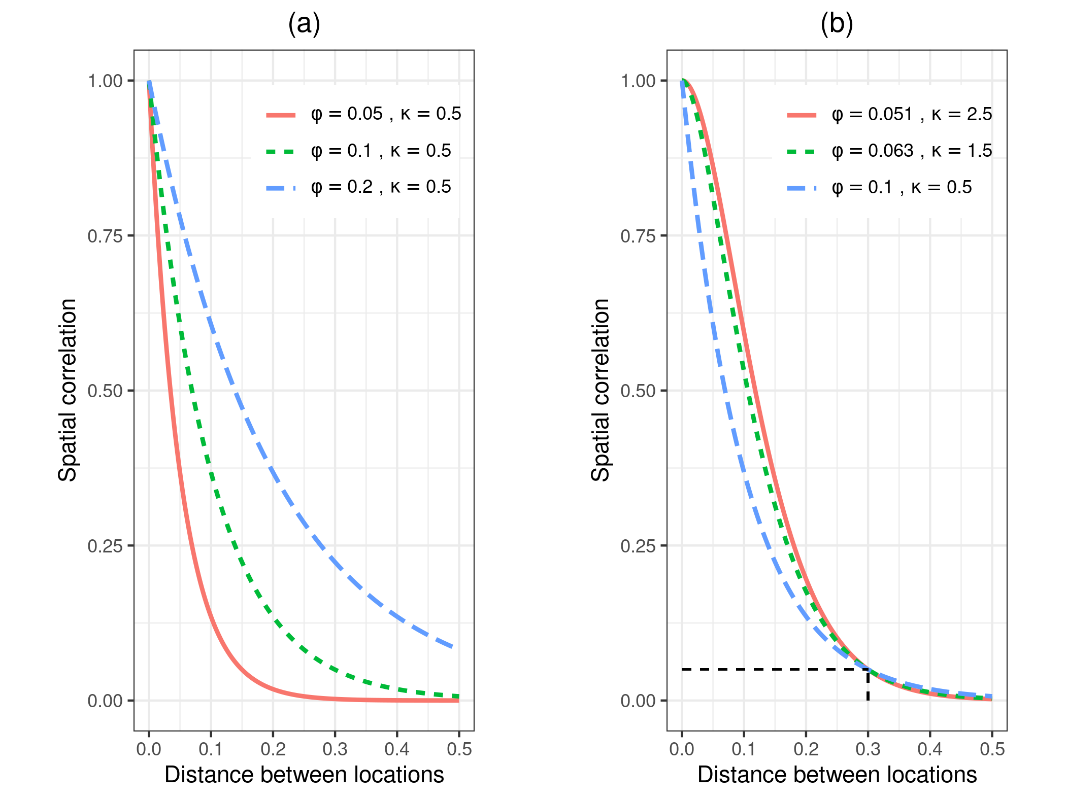
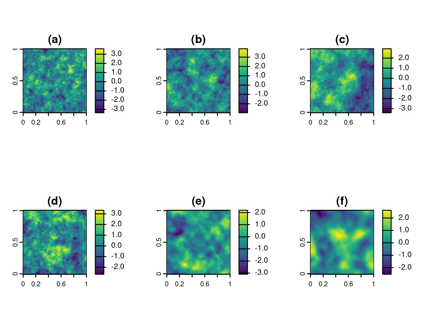
Figure 1.6 shows six different Matern correlation functions. In panel (a), we have kept \(\kappa\) fixed to 0.5 and varied \(\phi\) over the values 0.05, 0.1 and 0.2. For larger values of \(\phi\) the correlation function has a slower decay to zero. Panels (a) to (c), in Figure 1.7, show three realizations of a Gaussian process from each of these correlation functions. The mean of the Gaussian process was set to zero and variance to 1. We can observe that spatial correlations with larger scales are associated with longer spatial trends, whilst smaller scales exhibit a patchier pattern. This is because, as \(\phi\) takes values that are closer to zero, the spatial surface will tend to show a less structured pattern and will revert towards its zero mean more rapidly. In our examples in the book, we will often use the so called practical range to interpret our estimates for \(\phi\). The practical range is defined as the distance at which spatial correlation reaches 0.05, hence one can interpret this as the distance beyond which observations can be considered approximately independent. In the case of the exponential correlation function, the practical range is \(\log(20) \times \phi \approx 3 \phi\).
Finally, let us consider the correlation functions shown in panel (b) of Figure 1.6. Here, we vary \(\kappa\) over the values 0.5, 1.5, and 2.5, while keeping \(\phi\) fixed so that all three correlation functions reach 0.05 at a distance of 0.3. This setup allows us to isolate the effect of \(\kappa\) on the smoothness of the spatial process, while maintaining approximately the same correlation range across the three cases.
In Figure 1.7, we show three realizations from these correlation functions. We notice that smaller values of \(\kappa\) (e.g., \(\kappa = 0.5\)) produce rougher and less regular spatial patterns, whereas larger values (e.g., \(\kappa = 2.5\)) result in smoother and more continuous surfaces. These visual differences reflect the varying degrees of differentiability of the Gaussian process, which mathematically determines its local behavior and hence its smoothness.
Readers interested in the theoretical foundations of these properties may refer to Chapter 2 of Stein (1999).
The flexibility provided by the Matern correlation function in capturing different forms of spatial correlations has made it the most widely used correlation function in model-based geostatistics (Stein 1999). For this reason, in this book we will consider the Matern correlation function. We will consider estimation issues related to the Matern correlation in Chapter 3.
1.6 Workflow of a statistical analysis and structure of the book
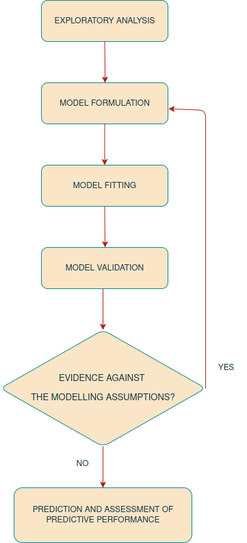
Figure 1.8 illustrates the stages involved in carrying out a geostatistical analysis of the examples introduced in Section 1.4. The process begins with exploratory data analysis, which is essential for understanding the empirical associations between risk factors and the health outcome of interest. In our case, this stage also helps justify the use of geostatistical models by questioning the assumptions underlying standard generalized linear models. The insights gained from this initial step guide the formulation of a suitable statistical model, whose parameters are then estimated using likelihood-based methods. This approach provides measures of uncertainty not only for the regression coefficients but also for the parameters that define the structure of spatial correlation in the data.
Once estimation has been carried out, the next step is model validation, where diagnostic tools are used to assess whether the fitted model can be trusted to represent the observed variation in the outcome. If the diagnostics indicate a poor fit, the process returns to the formulation stage to address the shortcomings revealed by the validation. If no evidence against the model is found, we move on to spatial prediction.
At this stage, defining appropriate predictive targets is crucial, as they ensure that the analysis answers the original research questions and supports decision making. An equally important component is evaluating how well the model predicts unobserved data, often referred to as predictive performance. In geostatistical applications, this evaluation is particularly challenging because spatial data are typically sparse and irregularly distributed. A widely used approach to quantify predictive performance is cross validation, which involves withholding a subset of observations, fitting the model to the remaining data, and then comparing the predictions to the held out observations. The design and interpretation of cross validation, however, depend on the ultimate goal of the analysis, for example whether the aim is to make predictions within the study region or to extrapolate beyond the sampled area. In addition to cross validation, simulation studies provide a valuable complementary tool, allowing us to better understand how a model should be expected to perform on average and to assess whether the results from a given analysis are consistent with this expected behaviour.
In the remainder of this book, each chapter focuses on one or more of these stages as shown in Figure 1.8. Chapter 2 introduces methods for working with spatial data in R, with a focus on raster and vector formats, including points and polygons. The skills developed in this chapter are applied throughout the book and are especially important in Chapter 4 and Chapter 5, where predictive maps of health outcomes are generated. Chapter 3 then describes the process of model formulation and estimation, showing how exploratory analyses inform the choice of model and how maximum likelihood methods can be used for parameter estimation. Chapter 4 builds on this by demonstrating how fitted models can be used for spatial prediction on both continuous and aggregated scales, and how predictive performance can be assessed to identify the most suitable model. Finally, Chapter 5 presents complete applications of all methods to three datasets, summarizing the full geostatistical workflow and illustrating additional features of the RiskMap R package not covered in earlier chapters.